§ 7.6 Module 7 — Matching and Optimising
Diameter Versus Energy: The Classic Trade
Pipe is purchased by diameter once. Friction is purchased by diameter every hour the pump runs.Module 7
By the end of this lesson
- Show why friction loss scales so strongly with diameter
- Find an economic diameter and describe the flatness of the optimum
- Explain how duty cycle changes the answer for a sewage station
7.6.1The fifth power hiding in Darcy-Weisbach
Darcy-Weisbach says hf = f(L/D)v²/(2g). At fixed flow, v = 4Q/(πD²), so substitution gives hf = 8fLQ²/(gπ²D⁵). Treat friction factor as slowly varying and loss scales approximately with the inverse fifth power of diameter. A 10% larger bore therefore gives roughly 1/1.1⁵ = 0.621 times the friction loss — about 38% less — before the smaller change in friction factor is recomputed.
That leverage is why a force main selected only by a maximum velocity can be expensive to own. It is also why internal diameter, not nominal size, belongs in the model: wall class, lining and material change the bore. Every candidate diameter needs a complete system curve and operating point, not a D⁻⁵ shortcut applied after pump selection.
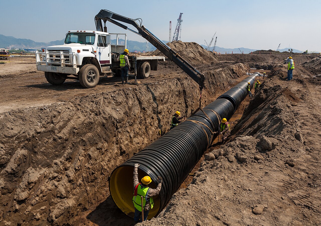
Diameter decisions become excavation, handling and jointing decisions in the field. The energy model prices the bore; the lifecycle comparison must also price how the main is actually built.
TomascastelazoCC BY-SA 3.0Wikimedia Commons
7.6.2One cost falls while another rises
Larger pipe costs more to buy and install: material, trench width, fittings, thrust restraint, valves and sometimes easement. Its energy present value falls because friction head falls. Add the two curves and a minimum appears. For each commercially available internal diameter, calculate installed cost, annual duty-bin energy, present value, renewals and any differential maintenance. The economic diameter is the least total among feasible sizes, not the unconstrained minimum of a smooth equation.
The simplified teaching model C(D) = A/D⁵ + BD² exposes the shape. Differentiating gives D* = (5A/2B)1/7. The seventh root makes the optimum move slowly: even a large change in energy price often shifts the continuous optimum modestly, and available nominal sizes then turn the answer into a small comparison table.
C(D) = 1/D⁵ + 5D²
D* = (5/(2×5))^(1/7) = 0.9057 normalized diameter
evaluate available sizes on BOTH sides; do not round first
the minimum is a region to understand, not a decimal to procure
A normalized cost curve near its continuous minimum.
Economic pipe sizing predates electronic optimization
Waterworks engineers compared annualized pipe and pumping costs long before spreadsheets, using tables, graphical cost curves and rules such as Bresse-type economic-velocity relations. Those rules encoded local prices and duty assumptions; they were never laws of fluid mechanics. Modern discounted cash flow makes the assumptions easier to expose, not less necessary.
Interactive lab bench
Find the shallow valley between pipe and power
A 3D instrument you drive yourself, one variable at a time. It needs JavaScript and WebGL, so it is not shown in this static copy of the page.
A lifecycle model can reward low velocity, long detention or an operating point outside the preferred region if those consequences were never given a cost or constraint.
Screen alternatives for hydraulic and operational acceptability before ranking the survivors by present value.
7.6.3The bottom is usually flatter than the argument around it
Report the cost premium of adjacent feasible sizes, not only the winner. If 300 mm is lowest at $2.41 million present value, 350 mm is $2.43 million and 250 mm is $2.58 million, the lower side is steep and the upper side is flat. The 350 mm option may be prudent under uncertain growth or energy price; the 250 mm option has little such defence. A flat minimum is information: it lets resilience, constructability and future uncertainty decide without pretending the arithmetic is more precise than its inputs.
Sensitivity should move energy price, pumped volume, discount rate, roughness at design age and service life. If one nominal size remains near-minimum across the matrix, the decision is robust. If the winner switches repeatedly, obtain better quantities and operating data, or explicitly price flexibility.
Check your understanding
Read the trade
1 auto-graded question with an explanation for every wrong answer. Requires JavaScript. (m7-l6-q1)
7.6.4Sewage duty cycle adds a lower-bound constraint
A sewage force main cannot be enlarged on energy alone. Greater diameter lowers velocity and may reduce the frequency or duration of scouring flow, increasing deposition and septicity risk. Minimum and scouring velocities are practice requirements set by the governing authority and must be named; they are not universal constants. Evaluate the actual pump cycle: how often each flow occurs, for how long, and whether duty rotation or periodic higher-flow operation provides the required transport.
Potable-water mains have different constraints: pressure range, water age, fire flow and storage operation. The economic calculation is common, but the feasible set is service-specific. This is the module's closing point: optimization never removes engineering constraints. It makes the cost of respecting them visible.
Lab 7.6
Find the continuous economic diameter
Write economicDiameter(energyCoefficient, capitalCoefficient) for C(D)=A/D⁵+B·D² . Return the positive diameter at minimum cost. Graded in the browser against 2 assertions; the editor and harness require JavaScript.
Examination score
The scorecard totals this page’s graded work as you go. It requires JavaScript.
The optimum is a shallow valley bounded by constraints, not a magic velocity.