§ 6.6 Module 6 — Pumps
Affinity Laws and Variable Speed
Speed moves the pump curve. It does not lower the hill.
By the end of this lesson
- Apply the affinity laws to predict performance at a new speed
- Show why static-dominated systems have a minimum useful speed
- Decide whether a VFD is justified for a given system curve
6.6.1Three exponents, one similarity assumption
For the same impeller handling the same liquid at geometrically similar points, the affinity laws give Q₂/Q₁ = N₂/N₁, H₂/H₁ = (N₂/N₁)², and P₂/P₁ = (N₂/N₁)³. Flow follows speed, head its square, and shaft power its cube.
speed ratio r = 1,350/1,800 = 0.75
Q₂ = 100 L/s × 0.75 = 75.0 L/s
H₂ = 40.0 m × 0.75² = 22.5 m
P₂ = 60.0 kW × 0.75³ = 25.31 kW
Reduce 1,800 rpm to 1,350 rpm
These relations move corresponding points on the pump curve. They do not guarantee the system will operate at 75 L/s, because the new pump curve must still intersect the unchanged system curve. Efficiency, motor/drive losses, minimum speed, cooling, vibration, and NPSH also limit useful range.
6.6.2Static head creates a speed floor
A system curve can be written Hs(Q) = Hstatic + kQ². Speed changes the pump curve; Hstatic remains the elevation difference between water surfaces. If the reduced-speed shutoff head falls below static lift, the pump has no forward-flow intersection at all.
For a full-speed shutoff head of 40.0 m and static lift of 25.0 m, the theoretical minimum speed ratio is √(25/40) = 0.7906. Below 79.1% speed, even shutoff head cannot reach the receiving surface. Real controls require margin above that limit and must respect the check valve and transient behaviour; the equality is a boundary, not an operating setpoint.
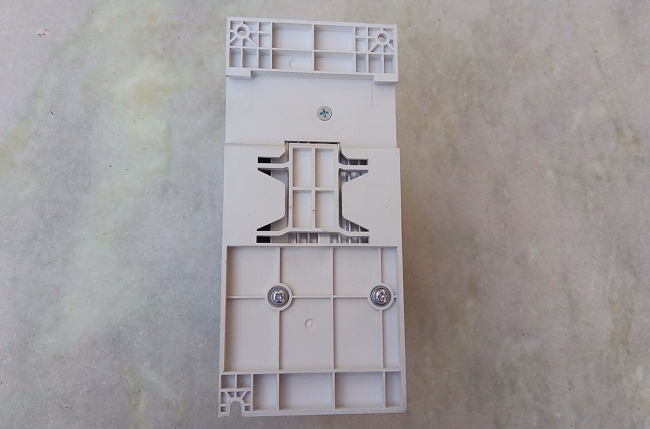
A variable-frequency drive is power electronics, cooling and protection hardware—not a free mathematical speed knob. Its enclosure, harmonics, bypass and failure mode belong in the station design.
Suyash.dwivediCC BY-SA 4.0Wikimedia Commons
Interactive lab bench
Turn down speed, not the hill
A 3D instrument you drive yourself, one variable at a time. It needs JavaScript and WebGL, so it is not shown in this static copy of the page.
Q ∝ N, H ∝ N², P ∝ N³ are correct, and they are the single most misapplied set of relations in pumping. They map one point on the pump curve to a corresponding point at a new speed, along a parabola through the origin. They say nothing about where the pump will actually operate, because that is set by the system curve.
On a system that is pure friction — no static lift — the system curve is also a parabola through the origin, the two coincide, and the affinity laws do predict the operating point. On a system with static lift they do not. Take a station with 20 m of static lift and 10 m of friction at design flow: drop the speed to 70% and the pump can no longer make 20 m at all. Flow does not fall to 70%, it falls to zero. The cube law on power, which is the entire energy-saving argument for a VFD, evaporates along with it.
Never quote VFD savings from the cube law on a station with meaningful static lift. Draw the system curve, walk the pump curve down in speed steps, and read the real operating points off the intersections — then compute power at each. §7.5 does this. On a high-static station the honest answer is often that a VFD saves very little and its real value is soft-start and level control.
6.6.3When a VFD saves energy
In a friction-dominated loop, reducing flow removes most of the required head, so the cubic power trend can be approached. In a static-dominated lift station, most head remains at low flow; speed has little room to fall before the curve loses its intersection. The US Department of Energy’s Variable Speed Pumping guide makes this system distinction explicit.
The correct comparison is annual energy at the expected operating distribution, including drive and motor efficiency, against throttling, on/off storage, staging, or a better-sized impeller. Include minimum scouring velocity for wastewater, motor cooling at low speed, harmonic and bypass requirements, control instrumentation, and the cost of added failure modes.
Control moved from valves to frequency
Throttling changes the system curve by wasting head across a valve. Electronic variable-frequency drives instead move the pump curve. That is an important efficiency gain when system friction falls with flow, but it cannot repeal a reservoir elevation.6.6.4A defensible variable-speed decision
- Draw the minimum, normal, and maximum system curves, separating static and friction head.
- Generate speed curves from certified data and find each operating intersection.
- Check every point against preferred region, NPSH margin, motor power, cooling, and minimum useful speed.
- Integrate wire power over the load-duration distribution, including drive losses.
- Compare against fixed-speed staging and impeller selection; state the control and bypass philosophy.
Check your understanding
Find the immovable term
1 auto-graded question with an explanation for every wrong answer. Requires JavaScript. (m6-l6-q1)
Lab 6.6
Implement the speed affinity laws
Write atSpeed(q1, h1, p1, n1, n2) returning {q2,h2,p2} . Graded in the browser against 2 assertions; the editor and harness require JavaScript.
Examination score
The scorecard totals this page’s graded work as you go. It requires JavaScript.
Head, Loss and Lift · Module 6, Lesson 6